Fix Slow Query: A Developer's Guide to Data Warehouse Performance
17 min readBY
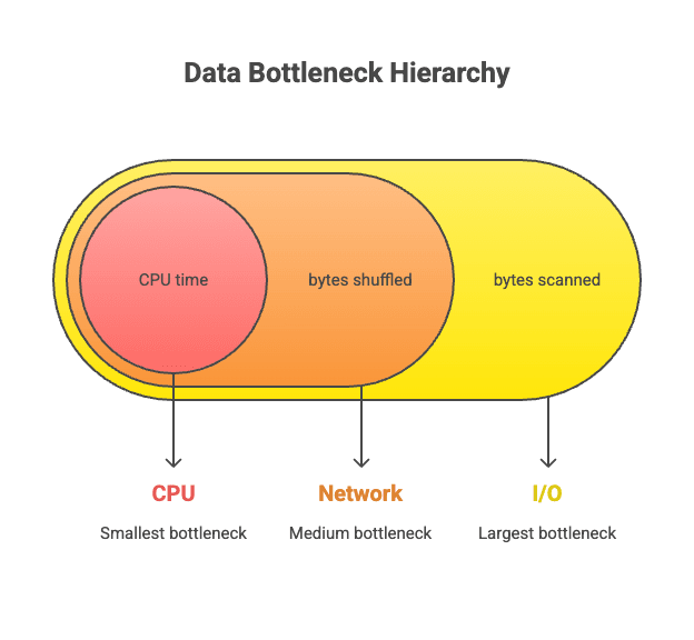
A developer pushes a new feature powered by a data warehouse query. In staging, it is snappy. In production, the user-facing dashboard takes five seconds to load, generating user complaints and performance alerts. This scenario is painfully common. The modern data stack promised speed and scale, yet developers constantly find themselves fighting inscrutable latency. Slow queries are not a vendor problem. They are a physics problem. Performance is governed by a predictable hierarchy of bottlenecks: reading data from storage (I/O), moving it across a network for operations like joins (Shuffle), and finally, processing it (CPU).
Without understanding this hierarchy, developers waste time optimizing the wrong things, such as rewriting SQL when the data layout is the issue. They burn money on oversized compute clusters and deliver poor user experiences. This article provides a developer-centric mental model to diagnose and fix latency at its source. By understanding the physical constraints of storage, network, and compute, you can build data systems that are not just fast, but predictably and efficiently so.
TL;DR
- Query performance is a physics problem, with bottlenecks occurring in a specific order: I/O (storage), then Network (shuffle), then CPU (compute). Fixing them in this order is the most effective approach.
- Your data layout strategy is your performance strategy. Columnar formats, optimal file sizes, partitioning, and sorting can cut the amount of data scanned by over 90%, directly targeting the largest bottleneck.
- Distributed systems impose a "shuffle tax." The most expensive operations are large joins and aggregations that move terabytes of data between nodes. Avoiding the shuffle is the key to fast distributed queries.
- There is no one-size-fits-all warehouse. A "Workload-Fit Architecture" matches the engine to the job's specific concurrency and latency needs, often leading to simpler, faster, and cheaper solutions for interactive workloads.
The Three-Layer Bottleneck Model: Why Queries Crawl
Latency is almost always I/O-bound first, then network-bound, then CPU-bound. A slow query is the result of a traffic jam in the data processing pipeline, and this congestion nearly always occurs in a predictable sequence across three fundamental layers. Developers often jump to optimizing SQL logic or scaling up compute clusters, which are CPU-level concerns. This is ineffective because the real bottleneck lies much earlier in the process: in the physical access of data from disk (I/O).
The hierarchy of pain begins with I/O. Reading data from cloud object storage like Amazon S3 is the slowest part of any query. An unoptimized storage layer can force an engine to read 100 times more data than necessary, a problem known as read amplification. Fixing data layout can yield greater performance gains than doubling compute resources.
Next comes the Network. In distributed systems, operations like joins and aggregations often require moving massive amounts of data between compute nodes in a process called the shuffle. This involves serialization, network transit, and potential spills to disk, making it orders of magnitude slower than memory access. The shuffle is a tax on distributed computing that must be minimized.
Finally, once the necessary data is located and moved into memory, the bottleneck becomes the CPU. At this stage, efficiency is determined by the engine's architecture. Modern analytical engines use vectorized execution, processing data in batches of thousands of values at a time instead of row-by-row, which dramatically improves computational throughput. Optimizing SQL is only impactful once the I/O and network bottlenecks have been resolved.
Scenario 1: Optimizing I/O for Slow Dashboards with Partitioning and Clustering
When a user-facing dashboard needs to fetch a small amount of data, such as sales for a single user, the query should be nearly instant. If it takes several seconds, the cause is almost always an I/O problem. The engine is being forced to perform a massive, brute-force scan to find a few relevant rows, a classic "needle in a haystack" problem. This occurs when the physical layout of the data on disk does not align with the query's access pattern.
The main culprits are partition and clustering misses. For example, a query filtering by user_id on a table partitioned by date forces the engine to scan every single date partition. Similarly, if data for a single user is scattered across hundreds of files, the engine must perform hundreds of separate read operations. The first time this data is read, it is a "cold cache" read from slow object storage, which carries the highest latency penalty.
The fix is to enable data skipping, where the engine uses metadata to avoid reading irrelevant data. Partitioning allows the engine to skip entire folders of data, while clustering (sorting) ensures that data for the same entity (like a user_id) is co-located in the same files. This allows the min/max statistics within file headers to be highly effective, letting the engine prune most files from the scan. This is addressed with features like Snowflake's Clustering Keys, BigQuery's Clustered Tables, Databricks' Z-Ordering, or Redshift's Sort Keys. Warehouses may also offer managed features to aid this, such as Snowflake's Search Optimization Service, which create index-like structures to accelerate these lookups at a cost.
From Theory to Practice: Implementing Data Layout
Understanding the need for a good data layout is the first step. Implementing it is the next. The most direct way to enforce clustering is to sort the data on write. Using SQL, you can create a new, optimized table by ordering the data by the columns you frequently filter on.
For example, to create a clustered version of a page_views table for fast user lookups:
Copy code
CREATE TABLE page_views_clustered AS
SELECT * FROM page_views
ORDER BY user_id, event_timestamp;
This physical ordering ensures that all data for a given user_id is stored contiguously, dramatically reducing the number of files the engine needs to read for a query like WHERE user_id = 'abc-123'.
For teams using dbt, this can be managed directly within a model's configuration block. This approach automates the process and keeps the data layout logic version-controlled alongside the rest of the data transformations.
Copy code
-- in models/marts/core/page_views.sql
{{
config(
materialized='table',
partition_by={
"field": "event_date",
"data_type": "date",
"granularity": "day"
},
cluster_by = ["user_id"]
)
}}
SELECT
...
FROM
{{ ref('stg_page_views') }}
This configuration tells the warehouse to partition the final table by day and then cluster (sort) the data within each partition by user_id, providing a highly efficient layout for user-facing dashboards.
Scenario 2: Fixing Slow Joins by Minimizing Network Shuffle
Large joins in distributed systems are slow because of the massive data movement required. This network bottleneck, known as the shuffle, is the tax paid for distributed processing. When joining two large tables, the engine must redistribute the data across the cluster so that rows with the same join key end up on the same machine. This involves expensive serialization, network transfer, and potential spills to disk if the data exceeds memory.
Distributed engines primarily use two join strategies. A Broadcast Join is used when one table is small (e.g., under a 10 MB default in Spark). The engine copies the small table to every node, allowing the join to occur locally without shuffling the large table. This is highly efficient. A Shuffle Join is used when both tables are large. Both tables are repartitioned across the network based on the join key. This is brutally expensive and is often the cause of a slow query. This is known as a Broadcast Join in Spark, but the concept of distributing a small dimension table in a Star Schema to all compute nodes is a fundamental optimization in all MPP systems, including Snowflake and Redshift.
The performance of a shuffle join is further degraded by two killers: data skew and disk spills. Data skew occurs when one join key contains a disproportionate amount of data, creating a "straggler" task that bottlenecks the entire job. Disk spills happen when a node runs out of memory and is forced to write intermediate data to slow storage, turning a memory-bound operation into a disk-bound one.
From Theory to Practice: Reading an Execution Plan
Diagnosing a slow join requires inspecting the query's execution plan, which is the primary diagnostic tool. You can find this in Snowflake's Query Profile, BigQuery's Query execution details, or by running an EXPLAIN command in Databricks. While graphical plans are helpful, understanding the textual output is a critical skill. Consider a simplified plan for a shuffle join:
Copy code
== Physical Plan ==
SortMergeJoin [left_key], [right_key], Inner
:- *(2) Sort [left_key ASC], false, 0
: +- Exchange hashpartitioning(left_key, 200)
: +- *(1) FileScan parquet table_A[left_key] Batched: true, DataFilters: [], Format: Parquet
+- *(4) Sort [right_key ASC], false, 0
+- Exchange hashpartitioning(right_key, 200)
+- *(3) FileScan parquet table_B[right_key] Batched: true, DataFilters: [], Format: Parquet
Here is how to interpret it:
- Spot the Shuffle: The
Exchangeoperator is the shuffle. It indicates that data is being repartitioned and sent across the network. If you see anExchangeon both sides of a join, it is a shuffle join. The absence of anExchangeon one side would suggest a more efficient broadcast join. - Identify the Scan: The
FileScanoperator shows where data is being read from storage. A well-optimized query will show partition filters here (e.g.,PartitionFilters: [isnotnull(date), (date = 2024-10-26)]), confirming that partition pruning is working. - Find the Join Algorithm: The
SortMergeJoinindicates the specific type of shuffle join. Another common type isShuffleHashJoin. The choice of algorithm can have performance implications, but the presence of theExchangeis the bigger red flag.
When a query is slow, look for large bytes shuffled or time spent in shuffle metrics associated with the Exchange operator. If one task within the Exchange stage takes much longer than others, it is a clear sign of data skew.
For cases where you know a table is small enough to be broadcast but the optimizer fails to choose that strategy, you can often provide a hint in the SQL.
Copy code
SELECT /*+ BROADCAST(country_lookup) */
e.event_id,
c.country_name
FROM
events AS e
JOIN
country_lookup AS c
ON e.country_code = c.country_code;
This hint forces the engine to broadcast the country_lookup table, avoiding a costly shuffle of the massive events table.
Scenario 3: Solving Read Amplification with Columnar Formats like Parquet
Reading an entire file to answer a query that needs only one column is the most wasteful I/O operation and a clear sign of a poorly chosen file format. This happens with row-oriented formats like CSV or JSON, which store data in rows. To get the value from a single column, the engine must read and discard all other columns in that row. This is a primary cause of read amplification.
The solution is to standardize on columnar formats like Apache Parquet. Parquet stores data in columns, not rows, which immediately enables column pruning. If a query is SELECT avg(price) FROM sales, the engine reads only the price column and ignores all others. This can reduce storage footprints by up to 75% compared to raw formats and is a cornerstone of modern analytics performance.
Parquet's efficiency goes deeper, with a metadata hierarchy that enables further data skipping. Files are divided into row groups (e.g., 128 MB chunks), and the file footer contains min/max statistics for every column in each row group. When a query contains a filter like WHERE product_category = 'electronics', the engine first reads the footer. If the min/max statistics for a row group show it only contains 'books' and 'clothing', the engine can skip reading that entire 128 MB chunk of data. For this to be effective, data should be sorted by frequently filtered columns before being written, which makes the min/max ranges tighter and more precise.
From Theory to Practice: Writing Optimized Parquet
Creating an optimized data layout is a data engineering task performed during ETL/ELT. For teams using frameworks like Apache Spark, the write logic is the control point for implementing partitioning, sorting, and file compaction. A common pattern is to repartition the data by a low-cardinality key (like date) and then sort within those partitions by a higher-cardinality key (like user ID).
Here is a PySpark example demonstrating this pattern:
Copy code
# Assuming 'df' is a Spark DataFrame with page view events
# Define output path and keys
output_path = "s3://my-bucket/page_views_optimized"
partition_key = "event_date"
cluster_key = "user_id"
(df
.repartition(partition_key)
.sortWithinPartitions(cluster_key)
.write
.mode("overwrite")
.partitionBy(partition_key)
.parquet(output_path)
)
This code snippet does three critical things:
repartition(partition_key): Groups data by the partition key, ensuring all data for a given date ends up on the same worker node before writing.sortWithinPartitions(cluster_key): Sorts the data on each worker byuser_id, making the min/max statistics in the resulting Parquet files highly effective for pruning.partitionBy(partition_key): Writes the data out to a directory structure like/event_date=2024-10-26/, which enables partition pruning at the folder level.
This approach produces well-structured, skippable Parquet files that form the foundation of a high-performance data lakehouse.
The Economics of Speed: Cost vs. Performance Trade-offs
In the real world, performance is not an absolute goal defined by synthetic data warehouse performance benchmarks. It is an economic decision. Engineers constantly balance query speed, compute cost, storage cost, and their own time. Without this context, performance advice remains academic and is insufficient for making business-justified architectural choices. Every optimization is a trade-off between paying now or paying later.
The most fundamental trade-off is between compute and storage. Optimizing data layout by sorting and compacting files is not free. It requires an upfront compute cost to perform the ETL/ELT job. This, in turn, may slightly increase storage costs if less efficient compression is used to favor faster reads. However, this one-time investment pays dividends over time by dramatically reducing the compute costs for every subsequent query that reads the data. A well-clustered table might cost $50 in compute to write but save thousands of dollars in query compute over its lifetime.
This economic model extends to managed features. When you enable a feature like Snowflake's Search Optimization Service or BigQuery's Clustering, you are making a conscious financial decision. You are agreeing to pay for the managed compute required to maintain an index-like structure and for the additional storage that structure consumes. In return, you avoid paying for massive, recurring compute costs from brute-force table scans. This is a sensible trade-off for high-value, frequently executed queries, but a poor one for ad-hoc analysis on cold data.
Finally, the human cost must be considered. An engineer's time is often the most expensive resource. Spending two weeks manually optimizing a data pipeline to shave 10% off a query's runtime might not be worth it if simply scaling up the virtual warehouse for ten minutes a day would achieve the same result for a fraction of the cost. The goal is to find the right balance, investing engineering effort in foundational layout optimizations that provide compounding returns and using compute resources flexibly to handle spiky or unpredictable workloads.
This economic reality leads to a crucial insight: if the primary performance killers for interactive queries are I/O latency from object storage and network shuffle, what if we could architect a system that bypasses them entirely for certain workloads? This is the central idea behind a modern, Workload-Fit Architecture.
The Solution: Adopting a Workload-Fit Architecture
Fixing common performance scenarios reveals a pattern: most problems are symptoms of an architectural mismatch. The era of using one massive, monolithic MPP warehouse for every job is over. It is often too complex and expensive for the task at hand. This leads to a more modern approach: Workload-Fit Architecture, which is the principle of matching the tool to the job's specific concurrency, latency, and cost requirements.
This approach explicitly re-evaluates the I/O, Network, and CPU trade-offs for a given workload.
- I/O: An in-process engine like DuckDB, running on a developer's laptop or a cloud VM, can use the local operating system's page cache and achieve extremely low-latency I/O from local SSDs. For "hot" data that fits on a single machine, this is orders of magnitude faster than fetching data from remote object storage.
- Network: The single biggest advantage of an in-process or single-node architecture is the complete elimination of the network shuffle tax. Joins and aggregations happen entirely in-memory or with spills to local disk, avoiding the expensive serialization and network transit inherent in distributed systems.
- CPU: Without the overhead of network serialization and deserialization, more CPU cycles are spent on productive, vectorized computation. This allows in-process engines to achieve incredible single-threaded performance.
MotherDuck is a prime example of this workload-fit philosophy. It combines the speed of DuckDB's local-first, in-process vectorized engine with the persistence and scalability of a serverless cloud backend. It is not designed for petabyte-scale ETL. Instead, it excels at the vast majority of workloads: powering interactive dashboards, enabling ad-hoc analysis, and serving data apps on datasets from gigabytes to a few terabytes, where low latency is critical and the overhead of a distributed MPP system is unnecessary. Read more in our documentation about MotherDuck's Architecture.
Decision Matrix: Matching Your Workload to the Right Engine
Choosing the right architecture requires evaluating your workload along two critical axes: the number of simultaneous users or queries (Concurrency) and the required response time (Latency SLA). This matrix provides a framework for selecting the appropriate engine type.
| Sub-Second (<1s) | Interactive (1-10s) | Reporting (>10s) | |
|---|---|---|---|
| Very High (1000+ users) | Real-time OLAP (ClickHouse, Druid) Specialized engines for user-facing analytics with high concurrency. | MPP Warehouse (Snowflake, BigQuery) Designed for enterprise BI with elastic scaling for thousands of users. | MPP Warehouse (Snowflake, BigQuery) Can scale out compute to handle massive batch reporting workloads. |
| Medium (10-100 users) | MotherDuck, ClickHouse Excellent for internal dashboards and data apps where latency is key for a team. | MotherDuck, DuckDB (large server) Ideal for interactive analysis by a team, providing speed without MPP overhead. | All Engines Most modern warehouses can handle this. Choice depends on cost and specific features. |
| Low (1-10 users) | DuckDB (local), MotherDuck Unparalleled speed for local analysis or embedded apps, with cloud persistence. | DuckDB, MotherDuck Perfect for individual data scientists or small teams exploring data. Fast and simple. | DuckDB, All Cloud Warehouses For a few users running long queries, any engine will work. DuckDB offers simplicity. |
Conclusion: Performance is a Data Engineering Choice
Slow queries are not a mystery but a result of understandable physical principles. The path to performance is through disciplined data engineering: fixing I/O first by optimizing data layout, then minimizing network shuffles, and finally, choosing an architecture that fits the workload's economic and technical requirements. Performance is not a feature you buy from a vendor. It is a characteristic you design into your system. By addressing bottlenecks in the right order, I/O, then Network, then CPU, you can systematically build data applications that are fast, efficient, and cost-effective.
Path Forward
- Analyze Your Own Query: Pick one of your slow queries and inspect its execution plan. Can you identify the bottleneck using the I/O-Network-CPU model? Look for signs of full table scans, large data shuffles, or disk spills.
- Audit Your Data Layout: Examine the physical layout of your most frequently queried table. Is it stored in Parquet? Are file sizes optimized between 128MB and 1GB? Is the data sorted by columns commonly used in filters?
- Consider Your Architecture: For your next interactive dashboard or data application project, evaluate if a Workload-Fit architecture could provide better performance and lower complexity than a traditional MPP warehouse. For many medium-data workloads, the answer is yes.
Start using MotherDuck now!
FAQS
Why does it take so long to show sales or page hits for a user?
This "needle in a haystack" problem is typically an I/O bottleneck, forcing the query engine to scan massive amounts of data just to find a few relevant rows for a single user. Optimizing your data layout with clustering and partitioning is the first step to enable data skipping and speed up these lookups. For workloads that demand consistently fast, interactive analytics, a modern data warehouse like MotherDuck leverages the power of DuckDB to deliver near-instant results for such queries.
How can we improve the speed of our data warehouse reports?
The most effective way to improve report speed is to tackle bottlenecks in order, starting with I/O by optimizing your data layout through partitioning and sorting. This dramatically reduces the amount of data scanned, which is the most common cause of slowness. Adopting a workload-fit architecture with a platform like MotherDuck can also provide a simpler, faster, and more cost-effective solution specifically for interactive reporting and analytics.
Why do I need to read entire files when querying large datasets?
Your query engine reads entire files when the data layout isn't optimized, preventing it from "skipping" irrelevant data blocks. Without proper sorting or clustering, the engine's metadata can't effectively prune files, forcing a brute-force scan. Platforms like MotherDuck, built on the high-performance DuckDB engine, are architected to maximize the benefits of a good data layout and minimize costly I/O operations.
How can I optimize performance when using direct queries in a data warehouse environment?
For direct queries in data apps, performance hinges on minimizing I/O latency by aligning your physical data layout with common query patterns. Using techniques like partitioning and clustering allows the engine to skip most of the data and return results in milliseconds. This is where a serverless data warehouse like MotherDuck excels, providing the low-latency query engine needed to power snappy, user-facing applications without complex infrastructure management.
Why are my large range joins taking so long to complete?
Large joins are often slow due to the "shuffle tax" in distributed data warehouses, where massive amounts of data must be moved across the network between compute nodes. This network transit is a major bottleneck, often orders of magnitude slower than in-memory processing. Modern architectures like MotherDuck, which leverages DuckDB's state-of-the-art join algorithms, can process these complex operations with greater efficiency and less reliance on costly data shuffling.
How does query latency affect product-led teams building data apps?
High query latency directly translates to a poor user experience, with slow dashboards and unresponsive features leading to user frustration and abandonment. For product-led teams, this lag undermines the value of their data apps and can trigger a flood of performance alerts. Building on a fast, serverless platform like MotherDuck is crucial for these teams, as it provides the performance foundation needed to deliver the snappy, interactive experiences users expect.
What are some ways to improve data system performance and handle multiple users efficiently?
Beyond optimizing data layout, a key strategy is to adopt a "Workload-Fit Architecture" that matches your query engine to your specific needs. For interactive analytics with many concurrent users, traditional batch-oriented warehouses can struggle. A modern, serverless solution like MotherDuck is specifically designed for these high-concurrency, low-latency workloads, ensuring consistently fast performance for all users without manual scaling.
Why might lakehouse architectures have high latency issues?
Lakehouse architectures often suffer from high latency because they query data directly on cloud object storage like S3, which is inherently slow for I/O. If the data layout isn't meticulously optimized with partitioning and sorting, queries are forced to scan far more data than necessary, causing significant delays. To overcome this, you can use a high-performance query engine like MotherDuck, which can sit on top of your data lake to provide the speed needed for interactive analysis.
What solutions perform well when joining large datasets across S3 or other cloud storage?
High-performance joins on cloud storage require an engine that can both minimize I/O and execute joins efficiently without a massive "shuffle tax." The key is an architecture that can intelligently read only the necessary data and process joins using modern, vectorized algorithms. Cloud data warehouses like MotherDuck are built on DuckDB's powerful engine, which excels at running complex analytical queries and joins directly against data in S3 with remarkable speed.
Why do analysts complain about slow “time-to-first-insight”?
A slow "time-to-first-insight" is a direct symptom of query latency caused by I/O and network bottlenecks in the data warehouse. When analysts wait minutes for queries to run, their creative and exploratory workflow is constantly interrupted, leading to frustration and reduced productivity. By using a platform like MotherDuck, which is optimized for rapid, interactive queries, teams can eliminate these delays and empower analysts to find insights in seconds, not minutes.