Working with Pandas DataFrames: A Practical Guide & Best Practices
15 min readBY
Introduction to DataFrames: A Practical Guide to Processing Large CSVs
It's 4:59 PM on a Friday when the Slack notification pops up: "Hey, just sent over that customer behavior data you needed. It's a 500MB CSV. Can you have insights by Monday?"
If you're still using basic Python lists and dictionaries for this task, you're making life harder than necessary. That's where DataFrames come in, possibly the most useful abstraction for working with structured data in the last decade. For data professionals, understanding DataFrames isn't just helpful, it's essential.
What You'll Learn in This Data Deep Dive
This post provides a practical, no-fluff introduction to DataFrames, focusing primarily on the Pandas implementation that's become ubiquitous in the Python ecosystem. It covers:
- What exactly is a DataFrame?
- Why DataFrames matter to your productivity and sanity
- Creating DataFrames from various data sources
- Core operations: Selecting, filtering, and inspecting data
- Basic data manipulation: Adding columns and transformations
The goal isn't to rehash the documentation, but to show you why these concepts matter in practice and provide code snippets you can adapt for real-world scenarios. Consider this your field guide to working effectively with tabular data. You could also follow the code used in this post on this notebook.
What is a DataFrame?
At its core, a DataFrame is a two-dimensional, size-mutable, potentially heterogeneous tabular data structure with labeled axes (rows and columns).
That's quite a mouthful, so let's break it down:
- Two-dimensional: DataFrames organize data in rows and columns, similar to a spreadsheet or database table. This maps naturally to how most structured data is represented.
- Size-mutable: Unlike fixed-size arrays, you can easily add or remove rows and columns after creating a DataFrame. This flexibility is invaluable during data cleaning and feature engineering.
- Potentially heterogeneous: Each column can store a different data type (integers, floats, strings, dates, etc.). This matches the reality of most datasets, which rarely contain uniform data types.
- Labeled axes: Both rows and columns have labels. Column labels are human-readable names describing each variable, while row labels form what's called the Index. This allows you to access data by name rather than just numeric position.
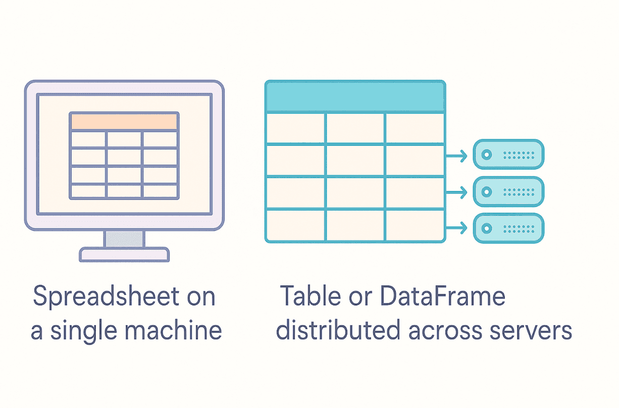
If tables are the bread and butter of data analysis, then DataFrames are the whole bakery. They provide a structured way to represent and work with virtually any tabular dataset you'll encounter in the wild.
Why Should I Use DataFrames?
So why add another data structure to your toolkit when Python already has lists, tuples, and dictionaries? Here are the key reasons DataFrames are indispensable:
- Natural Tabular Representation: DataFrames map directly to how we conceptualize structured data. Operations like selecting columns, filtering rows, or grouping data become much more intuitive.
- Rich Built-in Functionality: Need to calculate summary statistics? Handle missing values? Merge datasets? Reshape data? DataFrames come with built-in methods for these common tasks, saving you from writing boilerplate code.
- Performance Optimizations: Under the hood, libraries like Pandas use highly optimized C code (via NumPy) for many operations. This means calculations can be significantly faster than equivalent Python loops, especially on larger datasets.
- Ecosystem Integration: They play well with others. Reading data from CSVs, JSON, SQL databases, Excel files, or Parquet is typically straightforward. DataFrames also integrate well with visualization libraries and machine learning frameworks.
- Automatic Data Alignment: When performing operations between DataFrames, data is automatically aligned based on labels. This prevents subtle bugs that can occur when manually managing indices.
The first time you replace 50 lines of nested loops and dictionary transformations with three concise DataFrame operations that run in a fraction of the time, you'll be pleasantly surprised. It’s like watching your data quack into formation, finally making sense.
How to Create and Start Working with a Pandas DataFrame?
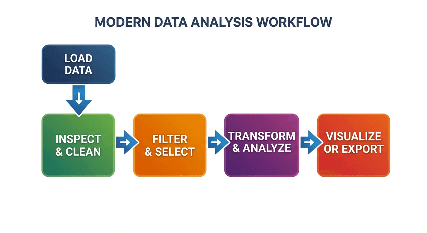
Common Pandas Workflow (Diagram)
To illustrate a typical process, here is a diagram showing the key stages of working with a DataFrame:
Time to get hands-on with some code. This section uses the ubiquitous Pandas library, which has become the de facto standard for data manipulation in Python.
If you don't have it installed, a quick pip install pandas will do the trick. The standard convention is to import it as pd:
Copy code
import pandas as pd
import numpy as np # Often used alongside pandas
Now, let's look at different ways to create a DataFrame. One common approach is using a Python dictionary where keys become column names and values become the column data:
Copy code
# --- Creating a DataFrame from a Dictionary ---
# Define the data as a dictionary
data_dict = {
'Engineer': ['Alice', 'Bob', 'Charlie', 'Diana'],
'Specialty': ['Backend', 'Data Infra', 'Frontend', 'Data Science'],
'YearsExp': [5, 8, 3, 6],
'HourlyRate': [95.0, 110.5, 80.0, 105.0]
}
# Create the DataFrame
df_engineers = pd.DataFrame(data_dict)
# Let's see what we've got!
print("--- DataFrame created from Dictionary ---")
print(df_engineers)
Code Explanation:
import pandas as pd: Imports the Pandas library with the conventional alias.data_dict = {...}: This code creates a standard Python dictionary.- The keys (
'Engineer','Specialty', etc.) will become column headers in the DataFrame. - The values are lists representing column data. All lists must have the same length for this method to work.
- The keys (
df_engineers = pd.DataFrame(data_dict): This creates the DataFrame, mapping keys to columns and lists to column data.print(df_engineers): Displays the resulting DataFrame, complete with the auto-generated integer index (0, 1, 2, 3).
Output:
Copy code
--- DataFrame created from Dictionary ---
Engineer Specialty YearsExp HourlyRate
0 Alice Backend 5 95.0
1 Bob Data Infra 8 110.5
2 Charlie Frontend 3 80.0
3 Diana Data Science 6 105.0
Another common pattern is creating a DataFrame from a list of dictionaries, where each dictionary represents a row:
Copy code
# --- Creating a DataFrame from a List of Dictionaries ---
# List where each dictionary is a row
data_rows = [
{'Metric': 'CPU Usage', 'Value': 0.75, 'Timestamp': '2025-04-25 09:30:00'},
{'Metric': 'Memory Usage', 'Value': 0.60, 'Timestamp': '2025-04-25 09:30:00'},
{'Metric': 'Disk IO', 'Value': 150.5, 'Timestamp': '2025-04-25 09:30:00'},
{'Metric': 'Network Traffic', 'Value': 5.2, 'Timestamp': '2025-04-25 09:30:00'}
]
# Create the DataFrame
df_metrics = pd.DataFrame(data_rows)
print("\n--- DataFrame created from List of Dictionaries ---")
print(df_metrics)
Code Explanation:
data_rows = [...]: This code creates a list where each element is a dictionary.- Each dictionary represents a row in the DataFrame.
- The keys become column headers, and Pandas infers columns from all keys present.
df_metrics = pd.DataFrame(data_rows): Again using the DataFrame constructor, but with different input structure.
Output:
Copy code
--- DataFrame created from List of Dictionaries ---
Metric Value Timestamp
0 CPU Usage 0.75 2025-04-25 09:30:00
1 Memory Usage 0.60 2025-04-25 09:30:00
2 Disk IO 150.50 2025-04-25 09:30:00
3 Network Traffic 5.20 2025-04-25 09:30:00
These examples only scratch the surface. You can also create DataFrames from NumPy arrays, lists of lists, or directly from files. For instance, reading from a CSV is as simple as:
Copy code
# Read directly from a CSV file
df = pd.read_csv('path/to/your/file.csv')
For more complex datasets, you might use an advanced analytical SQL engine like MotherDuck, which integrates smoothly with pandas for efficient data loading and transformation. This is particularly useful when working with large datasets that exceed memory constraints.
How Do I Inspect and Select Data from a DataFrame?
Once you have a DataFrame, you need to be able to explore and extract information from it.
How Can I Get a Quick Summary of My DataFrame?
The following examples use the df_engineers DataFrame to show some essential inspection commands:
Copy code
print("\n--- Inspecting the Engineers DataFrame ---")
# Display the first few rows (default is 5)
print("df_engineers.head(2):")
print(df_engineers.head(2))
# Display the last few rows (default is 5)
print("\ndf_engineers.tail(1):")
print(df_engineers.tail(1))
# Get concise summary (index dtype, column dtypes, non-null values, memory usage)
print("\ndf_engineers.info():")
df_engineers.info()
# Get descriptive statistics for numerical columns
print("\ndf_engineers.describe():")
print(df_engineers.describe())
# Get the dimensions (rows, columns)
print("\ndf_engineers.shape:")
print(df_engineers.shape)```
### Code Explanation & Output:
* `.head(n)`: Shows the first `n` rows. This is perfect for quickly glancing at your data structure:
```
df_engineers.head(2):
Engineer Specialty YearsExp HourlyRate
0 Alice Backend 5 95.0
1 Bob Data Infra 8 110.5
```
* `.tail(n)`: Shows the last `n` rows:
```
df_engineers.tail(1):
Engineer Specialty YearsExp HourlyRate
3 Diana Data Science 6 105.0
```
* `.info()`: Provides metadata about your DataFrame. This is a lifesaver for quickly spotting missing values or incorrect data types:
```
df_engineers.info():
<class 'pandas.core.frame.DataFrame'>
RangeIndex: 4 entries, 0 to 3
Data columns (total 4 columns):
# Column Non-Null Count Dtype
--- ------ -------------- -----
0 Engineer 4 non-null object
1 Specialty 4 non-null object
2 YearsExp 4 non-null int64
3 HourlyRate 4 non-null float64
dtypes: float64(1), int64(1), object(2)
memory usage: 256.0+ bytes
```
* `.describe()`: Generates summary statistics for numerical columns. This is an easy way to understand data distribution:
```
df_engineers.describe():
YearsExp HourlyRate
count 4.000000 4.00000
mean 5.500000 97.62500
std 2.081666 13.38765
min 3.000000 80.00000
25% 4.500000 91.25000
50% 5.500000 100.00000
75% 6.500000 106.37500
max 8.000000 110.50000
```
* `.shape`: Returns the dimensions as (rows, columns):
```
df_engineers.shape:
(4, 4)
```
### How Do I Select Columns?
Accessing specific columns is straightforward, similar to dictionary access:
```python
# Select a single column (returns a Pandas Series)
engineer_names = df_engineers['Engineer']
print("\n--- Selecting a Single Column ('Engineer') ---")
print(type(engineer_names))
print(engineer_names)
# Select multiple columns (returns a new DataFrame)
# Note the double square brackets! [[]]
experience_and_rate = df_engineers[['Specialty', 'HourlyRate']]
print("\n--- Selecting Multiple Columns ('Specialty', 'HourlyRate') ---")
print(type(experience_and_rate))
print(experience_and_rate)
Code Explanation:
df_engineers['Engineer']: Using single brackets selects one column, returning a PandasSeries(a 1D labeled array).df_engineers[['Specialty', 'HourlyRate']]: Using double brackets with a list of column names selects multiple columns, returning a newDataFrame.
Output:
Copy code
--- Selecting a Single Column ('Engineer') ---
<class 'pandas.core.series.Series'>
0 Alice
1 Bob
2 Charlie
3 Diana
Name: Engineer, dtype: object
--- Selecting Multiple Columns ('Specialty', 'HourlyRate') ---
<class 'pandas.core.frame.DataFrame'>
Specialty HourlyRate
0 Backend 95.0
1 Data Infra 110.5
2 Frontend 80.0
3 Data Science 105.0
How Do I Select Rows Using .loc and .iloc?
This is where things get interesting, and occasionally confusing for newcomers. Pandas provides two primary methods for selecting rows:
.loc: Selects based on labels (index names and column names).iloc: Selects based on integer position (like standard Python list indexing)
Let's see them in action:
Copy code
print("\n--- Selecting Rows using .loc (Label-based) ---")
# Select row with index label 1
row_1_loc = df_engineers.loc[1]
print("Row with label 1 (.loc[1]):")
print(row_1_loc)
# Select rows with labels 0 and 2
rows_0_2_loc = df_engineers.loc[[0, 2]]
print("\nRows with labels 0 and 2 (.loc[[0, 2]]):")
print(rows_0_2_loc)
# Select rows with labels 1 to 3 (inclusive) and specific columns
subset_loc = df_engineers.loc[1:3, ['Engineer', 'YearsExp']]
print("\nRows 1-3, Columns 'Engineer', 'YearsExp':")
print(subset_loc)
print("\n--- Selecting Rows using .iloc (Position-based) ---")
# Select row at position 1 (the second row)
row_1_iloc = df_engineers.iloc[1]
print("Row at position 1 (.iloc[1]):")
print(row_1_iloc)
# Select rows from position 1 up to (but not including) position 3
# AND columns at positions 0 and 2
subset_iloc = df_engineers.iloc[1:3, [0, 2]]
print("\nRows 1-2, Columns 0, 2 (.iloc[1:3, [0, 2]]):")
print(subset_iloc)
Key Differences to Remember:
.locis label-based: Slices include the end label (.loc[1:3]includes row with label 3).ilocis position-based: Slices exclude the end position (.iloc[1:3]excludes position 3)
This distinction trips up many developers. It's a common pitfall: spending an entire afternoon debugging a missing row only to realize .iloc was used instead of .loc.
How Do I Filter Rows Based on Conditions?
This is where DataFrames truly shine. You can filter rows based on conditions applied to column values:
Copy code
print("\n--- Filtering Rows (Boolean Indexing) ---")
# Find engineers with more than 5 years of experience
experienced_engineers = df_engineers[df_engineers['YearsExp'] > 5]
print("Engineers with > 5 YearsExp:")
print(experienced_engineers)
# Find Backend or Frontend engineers
specialty_mask = (df_engineers['Specialty'] == 'Backend') | (df_engineers['Specialty'] == 'Frontend')
backend_frontend = df_engineers[specialty_mask]
print("\nBackend or Frontend Engineers:")
print(backend_frontend)
# Find Data specialists earning > $100/hr
data_high_earners_mask = (df_engineers['Specialty'].str.contains('Data')) & (df_engineers['HourlyRate'] > 100)
data_high_earners = df_engineers[data_high_earners_mask]
print("\nData Specialists earning > $100/hr:")
print(data_high_earners)
Code Explanation:
df_engineers['YearsExp'] > 5: Creates a booleanSerieswithTruewhere the condition is met.df_engineers[boolean_mask]: Returns only rows where the mask isTrue.- For compound conditions:
- Use
&for logical AND - Use
|for logical OR - Use
~for logical NOT - Always wrap individual conditions in parentheses!
- Use
- String operations use the
.straccessor for powerful text manipulation.
Output:
Copy code
--- Filtering Rows (Boolean Indexing) ---
Engineers with > 5 YearsExp:
Engineer Specialty YearsExp HourlyRate
1 Bob Data Infra 8 110.5
3 Diana Data Science 6 105.0
Backend or Frontend Engineers:
Engineer Specialty YearsExp HourlyRate
0 Alice Backend 5 95.0
2 Charlie Frontend 3 80.0
Data Specialists earning > $100/hr:
Engineer Specialty YearsExp HourlyRate
1 Bob Data Infra 8 110.5
3 Diana Data Science 6 105.0
How Do I Add or Modify Columns in a DataFrame?
Adding new columns or modifying existing ones is typically straightforward:
Copy code
print("\n--- Adding/Modifying Columns ---")
# Add a new column with a scalar value (same value for all rows)
df_engineers['OnBench'] = False
print("Added 'OnBench' column:")
print(df_engineers)
# Add a new column based on calculation from existing columns
df_engineers['EstimatedAnnual'] = df_engineers['HourlyRate'] * 40 * 50 # 40 hrs/wk, 50 wks/yr
print("\nAdded 'EstimatedAnnual' column:")
print(df_engineers[['Engineer', 'HourlyRate', 'EstimatedAnnual']])
# Modify an existing column (e.g., give everyone a small raise)
df_engineers['HourlyRate'] = df_engineers['HourlyRate'] * 1.02
print("\nModified 'HourlyRate' (2% raise):")
print(df_engineers[['Engineer', 'HourlyRate']])
Code Explanation:
df['NewColumn'] = value: Creates a new column if it doesn't exist.- A scalar value (like
False) is applied to all rows. - A list or
Serieswith a matching index gets assigned row-by-row.
- A scalar value (like
df['ExistingColumn'] = new_value: Overwrites values in an existing column.
Output:
Copy code
--- Adding/Modifying Columns ---
Added 'OnBench' column:
Engineer Specialty YearsExp HourlyRate OnBench
0 Alice Backend 5 95.0 False
1 Bob Data Infra 8 110.5 False
2 Charlie Frontend 3 80.0 False
3 Diana Data Science 6 105.0 False
Added 'EstimatedAnnual' column:
Engineer HourlyRate EstimatedAnnual
0 Alice 95.0 190000.0
1 Bob 110.5 221000.0
2 Charlie 80.0 160000.0
3 Diana 105.0 210000.0
Modified 'HourlyRate' (2% raise):
Engineer HourlyRate
0 Alice 96.90
1 Bob 112.71
2 Charlie 81.60
3 Diana 107.10
Best Practices for Working with a Pandas DataFrame
Writing efficient, scalable, and readable code is the real challenge when working with a DataFrame. Here are a few best practices:
- Avoid Looping with Vectorized Operations: Use built-in vectorized operations instead of iterating through rows. They are orders of magnitude faster.
- Embrace Method Chaining: Chain methods together (e.g.,
df.dropna().query(...)) to make code more readable and prevent creating intermediate DataFrames that consume memory. - Optimize Data Types: Downcast numeric columns or convert text to the
categorydata type to drastically reduce memory usage. - Know When to Move to a More Powerful Engine: For datasets over a few gigabytes, even optimized Pandas code will struggle. This is when to offload the heavy lifting to a scalable backend like MotherDuck, which lets you query large datasets with SQL and pull down only the results you need into a manageable DataFrame.
Getting Your Ducks in a Row
This guide has covered quite a bit: what DataFrames are, why they're valuable, and how to perform fundamental operations like creating, inspecting, selecting, filtering, and modifying data.
This is honestly just scratching the surface. DataFrames offer much more power, including:
- Grouping and aggregation with
.groupby() - Merging and joining datasets
- Handling missing data
- Time series functionality
- Pivot tables and reshaping
But with the concepts covered here, you now have a solid foundation to start exploring these more advanced features as you need them. The beauty of DataFrames is that you can start simple and gradually use more sophisticated capabilities as your data challenges grow.
Anyone who has tackled a large-scale data project with raw Python dictionaries knows it can be painful, slow, and error-prone. The switch to DataFrames can cut development time in half and execution time by 90%. It's the kind of approach many wish they had been shown from day one.
But what happens when that 'mammoth CSV' is actually a 50GB Parquet file, or a collection of hundreds of files? This is where local memory becomes a bottleneck. For these scenarios, tools like MotherDuck provide a powerful next step. MotherDuck is a serverless analytics platform based on DuckDB that lets you query large datasets in the cloud and pull down just the results you need into a Pandas DataFrame. Instead of trying to load everything into memory, you can perform your heavy filtering and aggregations using SQL in the cloud and then continue your analysis in Pandas with a much more manageable dataset. It’s a great way to scale your data wrangling without overhauling your entire workflow.
So next time you're staring into the abyss of yet another mammoth CSV, remember that you've got powerful tools to help make sense of it all. Your data ducks will thank you for it.
Happy wrangling!
Start using MotherDuck now!
FAQS
What should I do if my dataset is too large for my computer's memory?
When a dataset is too large to fit into memory, you should avoid loading the entire file at once. Instead, use a serverless analytics tool like MotherDuck to query the data in the cloud. This allows you to perform heavy filtering and aggregations with SQL first, then pull only the smaller, manageable results into a Pandas DataFrame for further analysis.
How does a tool like MotherDuck work with Pandas?
MotherDuck acts as a powerful query engine for large datasets. Instead of loading a huge file with Pandas, you connect to MotherDuck, use SQL to select or aggregate the specific data you need, and then fetch only those results into a Pandas DataFrame. This "query-first" approach prevents memory errors and leverages a dedicated analytics engine for the heavy lifting.
When should I use MotherDuck instead of just Pandas?
You should use MotherDuck when your dataset is too large to fit into your computer's RAM. While Pandas requires loading all data into memory, MotherDuck can query massive datasets in the cloud and send only the smaller, processed results back to your Pandas DataFrame.
Is MotherDuck a replacement for Pandas?
No, MotherDuck is a complement to Pandas. The recommended workflow is to use MotherDuck for the initial, large-scale querying and aggregation of massive datasets, and then pull the manageable results into a Pandas DataFrame for more detailed, local analysis and visualization.
I’m using Pandas, but it’s too slow or runs out of memory. What’s a better alternative?
When Pandas struggles with large files, the issue is memory—it tries to load everything at once. The solution is not to replace Pandas, but to augment it. A tool like MotherDuck allows you to use SQL to query the massive file in the cloud first, then load only the smaller, manageable results into a Pandas DataFrame for your analysis.
How do I handle missing values in a Pandas DataFrame?
The most common methods are df.dropna() to remove rows with any missing values, or df.fillna(value) to replace NaN values with a specific value (like 0, the mean, or the median). For time-series data, you can also use methods like ffill (forward fill) or bfill (backward fill).
What's the most efficient way to merge two DataFrames?
Always use the pd.merge() function with the on parameter specifying the key column(s). To avoid errors, ensure the key columns have the same name and data type in both DataFrames. If they have different names, use the left_on and right_on parameters.
How can I reduce the memory usage of my DataFrame?
First, use df.info() to see column data types. Use the astype() method to downcast numerical columns to more memory-efficient types (e.g., float32 instead of float64). For columns with a low number of unique string values, converting them to the category dtype with df['column'].astype('category') can lead to significant memory savings.