What We'll Build

By the end of this tutorial, you'll have:

• An interactive visualization of text embeddings in 2D - skip to the demo!
• Automatic clustering of similar texts
• The ability to explore relationships between different pieces of text
• A foundation for building your own text analysis tools

Setting Up Your Environment

You'll need:

• A MotherDuck account, with access to the embedding() function (a SQL function that converts text to embeddings)
• marimo locally installed. First, create a new virtual environment with your preferred package manager. Install with: pip install 'marimo[recommended]'or follow the installation instructions.
• Python >= 3.10

Create a new marimo notebook by running marimo edit embeddings_explorer.py. We'll start by importing the required libraries:

Copy code
# Data manipulation and database connections
import polars as pl
import duckdb
import numba # <- FYI, this module takes a while to load, be patient
import pyarrow

# Visualization
import altair as alt
import marimo as mo

# ML tools for dimensionality reduction and clustering
import umap  # For reducing high-dimensional embeddings to 2D
import hdbscan  # For clustering similar embeddings
import numpy as np
from sklearn.decomposition import PCA

marimo will automatically ask you to install these dependencies. Choose the package manager you used to install marimo from the dropdown and hit Install. If you would like to start from a reproducible notebook with the same versions, you can download this notebook and run: marimo edit embeddings_explorer.py --sandbox

Connecting to MotherDuck and Loading Sample Data

First, let's connect to MotherDuck. marimo supports both Python and SQL cells, making database operations straightforward:

Copy code
-- This will prompt you to log in and authorize the connection.
ATTACH IF NOT EXISTS 'md:my_db'

This command will open a new browser window to log into MotherDuck. Next, we'll load sample data from the Hacker News Posts dataset. We'll create a table called demo_embedding containing popular posts with a specific keyword. Thanks to marimo's reactivity, any changes to this query will automatically update (or mark stale) any dependent visualizations:

Copy code
CREATE OR REPLACE TABLE my_db.demo_embedding AS
SELECT DISTINCT ON (url) *  -- Remove duplicate URLs
FROM 'hf://datasets/julien040/hacker-news-posts/story.parquet'
WHERE contains(title, 'database')  -- Filter for posts about databases
    AND score > 5  -- Only include popular posts
LIMIT 50000;

Converting Text to Embeddings

Text embeddings are dense vectors that represent the meaning of text. Similar texts will have similar vectors, making them useful for tasks like semantic search and clustering. We'll use MotherDuck's embedding() function to generate these vectors:

Copy code
embeddings = mo.sql(
    f"""
 SELECT *, embedding(title) as text_embedding
 FROM my_db.demo_embedding
 LIMIT 1500;  -- Limiting for performance in this demo, but you can adjust this
 """
)

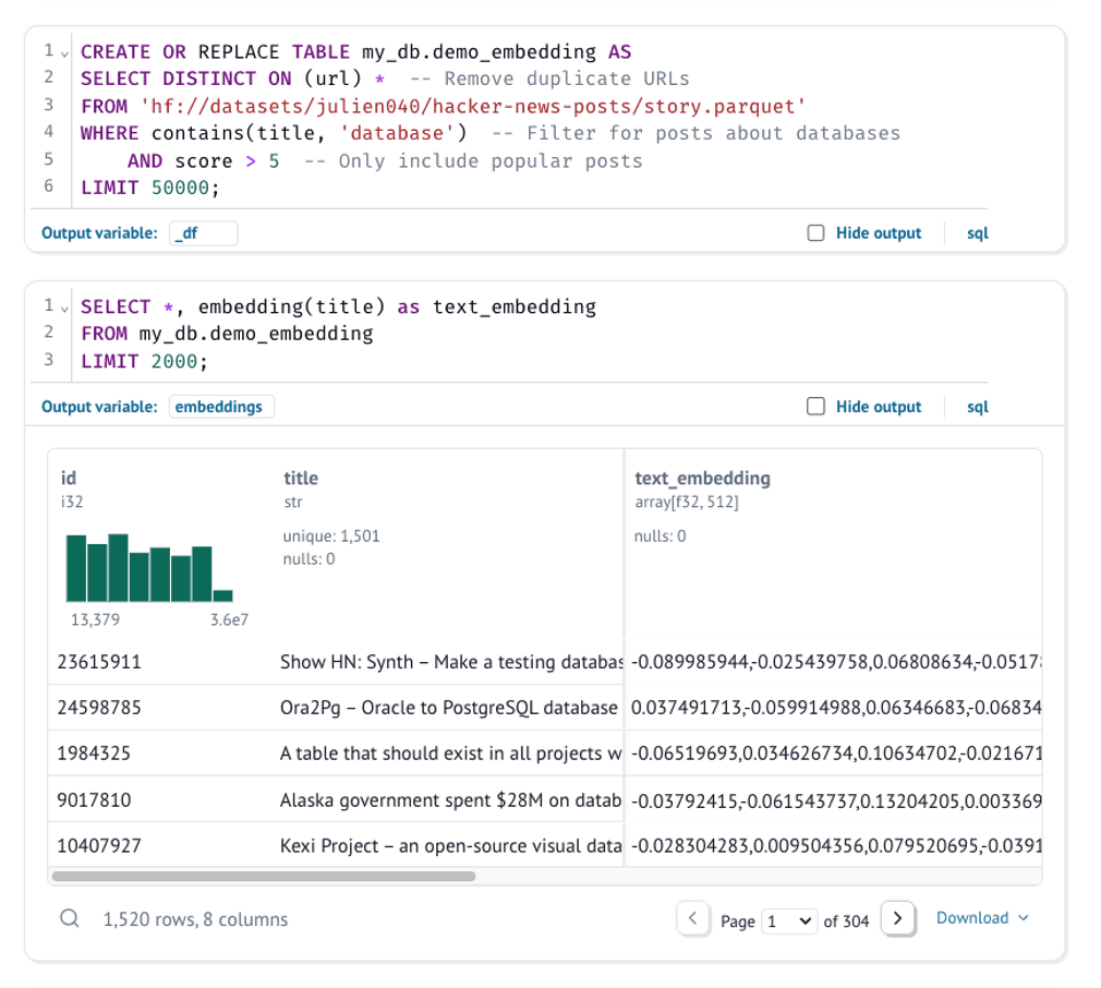
The results are stored in the embeddings variable in Python, which we'll use for clustering and visualization. Each embedding is a high-dimensional vector (in our case, 512 dimensions).

Making Sense of High-Dimensional Data

Text embeddings typically have hundreds of dimensions (512 in our case), making them impossible to visualize directly. We'll use two techniques to make them interpretable:

1. Dimensionality Reduction: Convert our 512D vectors into 2D points while preserving relationships between texts
2. Clustering: Group similar texts together into clusters

Here are our helper functions:

Copy code
def reduce_dimensions(np_array):
    """
    Reduce the dimensions of embeddings to a 2D space.

    Here we use the UMAP algorithm. UMAP preserves both local and
    global structure of the high-dimensional data.
    """
    reducer = umap.UMAP(
        n_components=2,  # Reduce to 2D for visualization
        metric="cosine",  # Use cosine similarity for text embeddings
        n_neighbors=80,  # Higher values = more global structure
        min_dist=0.1,  # Controls how tightly points cluster
    )
    return reducer.fit_transform(np_array)


def cluster_points(np_array, min_cluster_size=4, max_cluster_size=50):
    """
    Cluster the embeddings.
    Here we use the HDBSCAN algorithm. We first reduce dimensionality to 50D with
    PCA to speed up clustering, while still preserving most of the important information.
    """
    pca = PCA(n_components=50)
    np_array = pca.fit_transform(np_array)

    hdb = hdbscan.HDBSCAN(
        min_samples=3,  # Minimum points to form dense region
        min_cluster_size=min_cluster_size,  # Minimum size of a cluster
        max_cluster_size=max_cluster_size,  # Maximum size of a cluster
    ).fit(np_array)

    return np.where(hdb.labels_ == -1, "outlier", "cluster_" + hdb.labels_.astype(str))

Processing the Data

Now we'll transform our high-dimensional embeddings into something we can visualize:

Copy code
with mo.status.spinner("Clustering points...") as _s:
    embeddings_array = embeddings["text_embedding"].to_numpy()
    hdb_labels = cluster_points(embeddings_array)
    _s.update("Reducing dimensionality...")
    embeddings_2d = reduce_dimensions(embeddings_array)

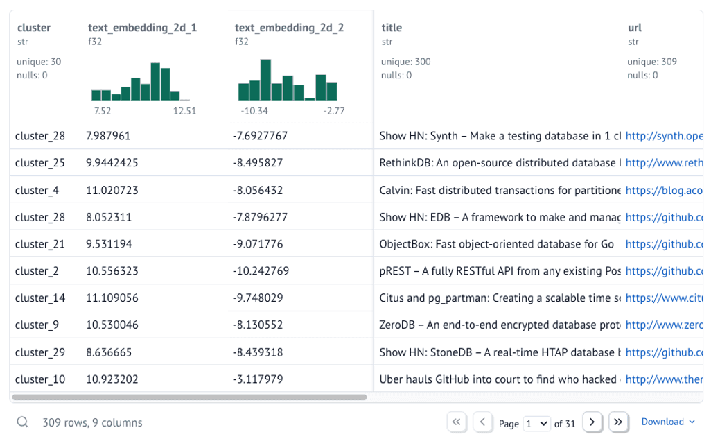
Using polars, we can stitch the 2D embeddings and the cluster labels back on to our original dataframe.

Copy code
data = embeddings.lazy()  # Lazy evaluation for performance
data = data.with_columns(
    text_embedding_2d_1=embeddings_2d[:, 0],
    text_embedding_2d_2=embeddings_2d[:, 1],
    cluster=hdb_labels,
)
data = data.unique(subset=["url"], maintain_order=True)  # Remove duplicate URLs
data = data.drop(["text_embedding", "id"])  # Drop unused columns
data = data.filter(pl.col("cluster") != "outlier")  # Filter out outliers
data = data.collect()  # Collect the data
data

Creating an Interactive Visualization

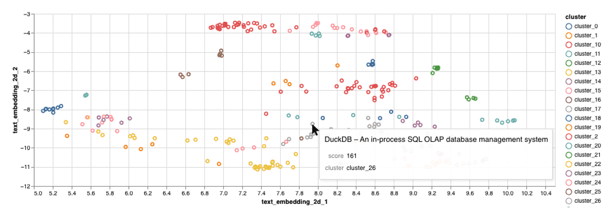
Let's create a scatter plot where:

• Each point represents a text (Hacker News title in our case)
• Similar texts appear closer together
• Colors indicate different clusters of related texts
• You can interact with points to see the underlying text

Copy code
chart = alt.Chart(data).mark_point().encode(
    x=alt.X("text_embedding_2d_1").scale(zero=False),
    y=alt.Y("text_embedding_2d_2").scale(zero=False),
    color="cluster",
    tooltip=["title", "score", "cluster"]
)
chart = mo.ui.altair_chart(chart)
chart

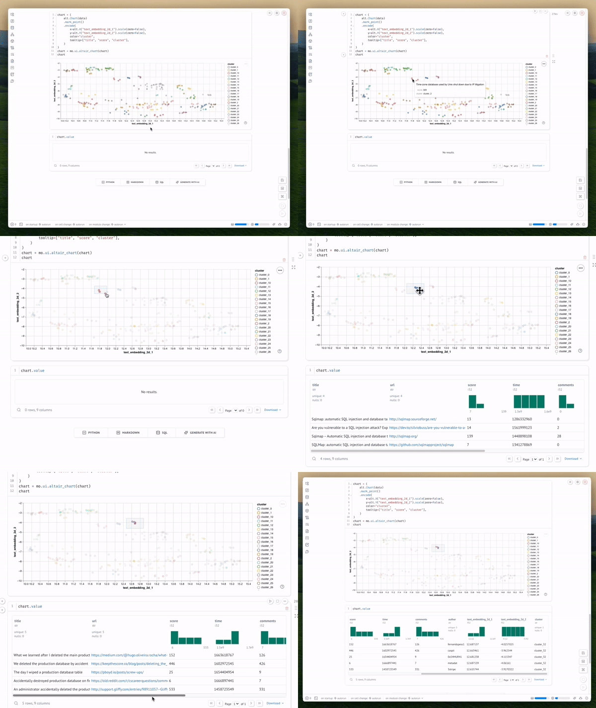
And display the chart's selected points:

Copy code
chart.value

Exploring the Results

You can interact with the visualization in several ways:

• Hover over points to see the actual titles
• Look for clusters of related topics
• Identify outliers or unexpected groupings

The visualization shows clusters of semantically similar texts. Each point represents a document, and the proximity between points indicates semantic similarity. Colors represent different clusters identified by our clustering algorithm.

Customizing the Analysis

You can experiment with:

1. UMAP parameters:
   • n_neighbors: Higher values (>100) preserve more global structure, lower values (<20) focus on local relationships
   • min_dist: Controls how tightly points cluster together
2. HDBSCAN parameters:
   • min_cluster_size: Minimum number of points to form a cluster
   • min_samples: Controls noise sensitivity (higher values = more points labeled as noise)
3. Different embedding models in MotherDuck:
   • Try embedding(title, model="text-embedding-3-large") for potentially better results

Next Steps

That's it! You've created an interactive text embedding explorer using MotherDuck and marimo. The full code is available here, as well as an interactive demo deployed as a marimo application.

If you prefer using python directly, its easy as these two commands to get started:

Copy code
pip install marimo
marimo edit

Some ideas if you’d like extend this:

• Change the initial dataset
• Choose a different initial keyword or filters
• Add marimo sliders and inputs to make tweaking UMAP and HDBSCAN even easier
• Implement semantic search functionality to highlight related points